VCT 2023 Champions Analysis

Probability a team wins a map

Posted on August 2023

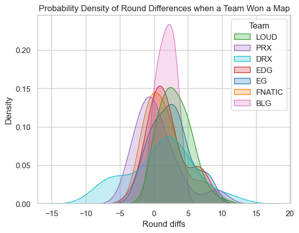
I am interested in finding the probability of a team win a map in VCT Champions. Prior to this, I realized that Paperrex (PRX), usually perform a comeback and won a map. So, I want to analyze the probability of a team won a map based on their round difference.

import pandas as pd
import numpy as np
import seaborn as sns
import matplotlib.pyplot as plt
from IPython.display import Image, display
from matplotlib.offsetbox import OffsetImage, AnnotationBbox

data_path = "VCT2023_rounddiffs_team_map_playoff_data.xlsx"

df = pd.read_excel(data_path, index_col=None)
df.head()

	Team	Round diffs	Map
0	LOUD	0	Ascent
1	LOUD	1	Ascent
2	LOUD	2	Ascent
3	LOUD	3	Ascent
4	LOUD	4	Ascent

df.dtypes

Team           object
Round diffs     int64
Map            object
dtype: object

sns.set_theme(style='whitegrid')
palette = {"LOUD":"tab:green",
           "PRX":"tab:purple",
           "DRX":"tab:cyan",
           "EDG":"tab:red",
           "EG":"tab:blue",
           "FNATIC":"tab:orange",
           "BLG":"tab:pink"}
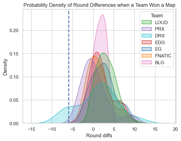
sns.kdeplot(data=df, x="Round diffs", hue="Team", fill=True, common_norm=False, palette=palette).set(title="Probability Density of Round Differences when a Team Won a Map")

[Text(0.5, 1.0, 'Probability Density of Round Differences when a Team Won a Map')]

png

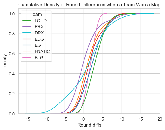
sns.kdeplot(data=df, x="Round diffs", hue="Team", cumulative=True, common_norm=False, palette=palette).set(title="Cumulative Density of Round Differences when a Team Won a Map")

[Text(0.5, 1.0, 'Cumulative Density of Round Differences when a Team Won a Map')]

png

Probability a team win the map when they have negative round differences

To obtain the probability, I used kernel density estimation to estimate the distribution of teams winning a map based on their round difference. Then I caculate the area under the curve that is less than 0.

# Probability winning a negative round diffs
teams = df["Team"].unique()
probability = []

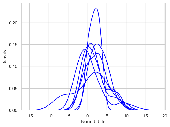
for team in teams:
  ax = sns.kdeplot(data=df[df["Team"] == team], x="Round diffs",common_norm=False, color="blue")
  # Get all the lines used to draw the density curve
  kde_lines = ax.get_lines()[-1]
  kde_x, kde_y = kde_lines.get_data()

  # Mask area under the curve that less than 0
  mask = kde_x < 0
  filled_x, filled_y = kde_x[mask], kde_y[mask]

  # Area of less than 0
  area = np.round(np.trapz(filled_y, filled_x)*100, 2)
  probability.append(area)

png

result = pd.DataFrame([teams, probability]).T
result.columns = ["Team", "Probability a team win the map when they have negative round differences (in %)"]
result.sort_values(by="Probability a team win the map when they have negative round differences (in %)", ascending=False, inplace=True)
fig, ax = plt.subplots(figsize=(10, 6))
ax = sns.barplot(data=result, x="Probability a team win the map when they have negative round differences (in %)", y="Team", palette=palette)

images = [plt.imread(team + ".png") for team in result["Team"]]
tick_labels = ax.yaxis.get_ticklabels()

ax.set(yticklabels=[])
ax.set(xticklabels=[])
ax.set(ylabel=None)
ax.grid(False)

for i in ax.containers:
    ax.bar_label(i,)

for i,image in enumerate(images):
    ib = OffsetImage(image, zoom=.15)
    ib.image.axes = ax
    ab = AnnotationBbox(ib,
                    tick_labels[i].get_position(),
                    frameon=False,
                    box_alignment=(1.25, 0.5)
                    )
    ax.add_artist(ab)

png

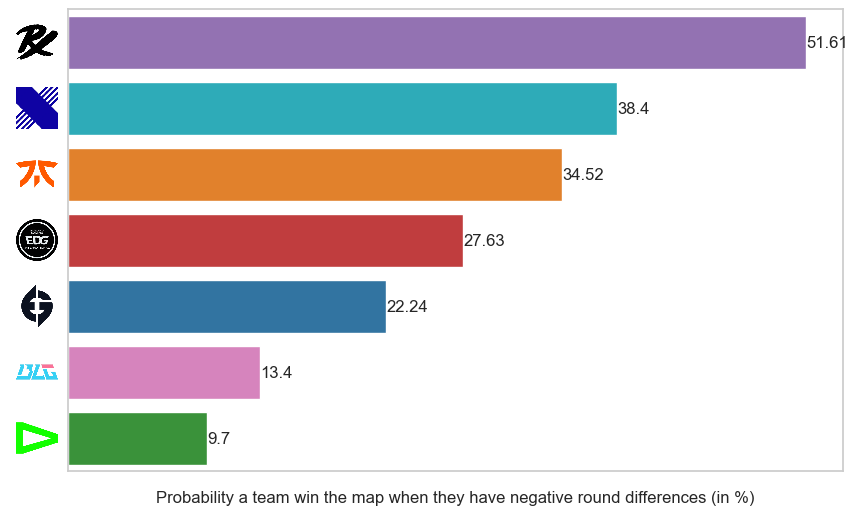
In general as I hypothesize earlier, PRX has the highest probability to win a map when they down a round followed by DRX.

Probability a team win the map when they have -6 round differences

# Probability winning a -6 round difference
teams = df["Team"].unique()
probability = []

for team in teams:
  ax = sns.kdeplot(data=df[df["Team"] == team], x="Round diffs",common_norm=False, color="blue")
  # Get all the lines used to draw the density curve
  kde_lines = ax.get_lines()[-1]
  kde_x, kde_y = kde_lines.get_data()

  # Mask area under the curve that less than -6
  mask = kde_x < -6
  filled_x, filled_y = kde_x[mask], kde_y[mask]

  # Area of less than -6
  area = np.round(np.trapz(filled_y, filled_x)*100, 2)
  #print("The probability that {} won a map when experiences 9-3 curse is: {}%".format(team, area))
  probability.append(area)

png

sns.set_theme(style='whitegrid')
sns.kdeplot(data=df, x="Round diffs", hue="Team", fill=True, common_norm=False, palette=palette).set(title="Probability Density of Round Differences when a Team Won a Map")
plt.axvline(x=-6, linewidth=2, linestyle='--')

<matplotlib.lines.Line2D at 0x29be734c990>

png

result = pd.DataFrame([teams, probability]).T
result.columns = ["Team", "Probability a team win the map when they down 6 rounds (in %)"]
result.sort_values(by="Probability a team win the map when they down 6 rounds (in %)", ascending=False, inplace=True)
ax = sns.barplot(data=result, x="Probability a team win the map when they down 6 rounds (in %)", y="Team", palette=palette)

images = [plt.imread(team + ".png") for team in result["Team"]]
tick_labels = ax.yaxis.get_ticklabels()

ax.set(yticklabels=[])
ax.set(xticklabels=[])
ax.set(ylabel=None)
ax.grid(False)

for i in ax.containers:
    ax.bar_label(i,)

for i,image in enumerate(images):
    ib = OffsetImage(image, zoom=.15)
    ib.image.axes = ax
    ab = AnnotationBbox(ib,
                    tick_labels[i].get_position(),
                    frameon=False,
                    box_alignment=(1.25, 0.5)
                    )
    ax.add_artist(ab)

png

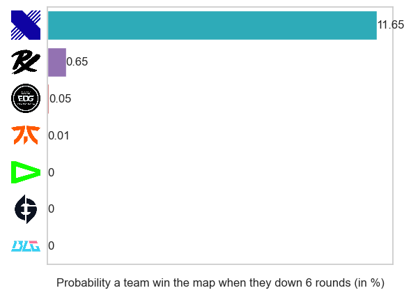
However, when we consider a “comeback” though (here I defined a comeback as winning with less than -6 round differences), DRX takes the spot. However, DRX is skewed because they have one match against BLG in which they comeback from -10 round differences.