Recurrent Neural Network with PyTorch
Implemention of recurrent neural network to forecast company revenue using PyTorch
Posted on: January 2024
Below is an implementation of recurrent neural network (RNN) with PyTorch to forecast the revenue of certain a company from 2015 to 2020.
The data is taken from here.
import pandas as pd
import numpy as np
import matplotlib.pyplot as plt
import matplotlib.ticker as ticker
import torch
data_path = '/content/drive/MyDrive/Colab Notebooks/data/Time Series Starter Dataset/Month_Value_1.csv'

df = pd.read_csv(data_path)
df
| Period | Revenue | Sales_quantity | Average_cost | The_average_annual_payroll_of_the_region | |
|---|---|---|---|---|---|
| 0 | 01.01.2015 | 1.601007e+07 | 12729.0 | 1257.763541 | 30024676.0 |
| 1 | 01.02.2015 | 1.580759e+07 | 11636.0 | 1358.507000 | 30024676.0 |
| 2 | 01.03.2015 | 2.204715e+07 | 15922.0 | 1384.697024 | 30024676.0 |
| 3 | 01.04.2015 | 1.881458e+07 | 15227.0 | 1235.606705 | 30024676.0 |
| 4 | 01.05.2015 | 1.402148e+07 | 8620.0 | 1626.621765 | 30024676.0 |
| ... | ... | ... | ... | ... | ... |
| 91 | 01.08.2022 | NaN | NaN | NaN | NaN |
| 92 | 01.09.2022 | NaN | NaN | NaN | NaN |
| 93 | 01.10.2022 | NaN | NaN | NaN | NaN |
| 94 | 01.11.2022 | NaN | NaN | NaN | NaN |
| 95 | 01.12.2022 | NaN | NaN | NaN | NaN |
96 rows × 5 columns
Remove empty data
df = df.dropna()
df
| Period | Revenue | Sales_quantity | Average_cost | The_average_annual_payroll_of_the_region | |
|---|---|---|---|---|---|
| 0 | 01.01.2015 | 1.601007e+07 | 12729.0 | 1257.763541 | 30024676.0 |
| 1 | 01.02.2015 | 1.580759e+07 | 11636.0 | 1358.507000 | 30024676.0 |
| 2 | 01.03.2015 | 2.204715e+07 | 15922.0 | 1384.697024 | 30024676.0 |
| 3 | 01.04.2015 | 1.881458e+07 | 15227.0 | 1235.606705 | 30024676.0 |
| 4 | 01.05.2015 | 1.402148e+07 | 8620.0 | 1626.621765 | 30024676.0 |
| ... | ... | ... | ... | ... | ... |
| 59 | 01.12.2019 | 5.875647e+07 | 38069.0 | 1543.420464 | 29878525.0 |
| 60 | 01.01.2020 | 5.628830e+07 | 27184.0 | 2070.640850 | 29044998.0 |
| 61 | 01.02.2020 | 4.022524e+07 | 23509.0 | 1711.057181 | 29044998.0 |
| 62 | 01.03.2020 | 5.002217e+07 | 32569.0 | 1535.882748 | 29044998.0 |
| 63 | 01.04.2020 | 5.232069e+07 | 26615.0 | 1965.834790 | 29044998.0 |
64 rows × 5 columns
Plot the data
fig, ax = plt.subplots()
ax.plot(df['Period'], df['Revenue'])
plt.xticks(rotation=90)
ax.xaxis.set_major_locator(ticker.MultipleLocator(base=6))
plt.title("Revenue")
Text(0.5, 1.0, 'Revenue')
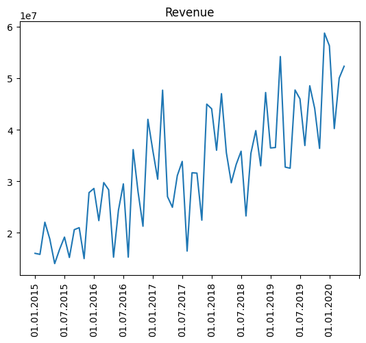
data = df['Revenue']
date = df['Period']
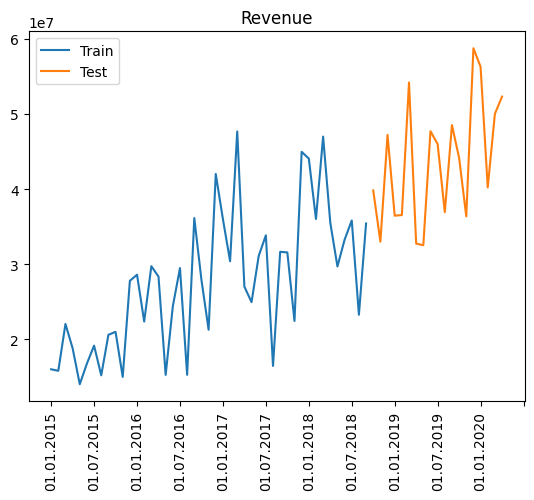
In this case, the data is divided into two categories: train and test. The composition of the train data is 70% of cleaned data while the other 30% is the test data.
train_len = int(round(0.7*len(data), 0))

train = data[:train_len]
test = data[train_len:]
train_index = date[:train_len]
test_index = date[train_len:]
fig, ax = plt.subplots()
ax.plot(train_index, train.values, label="Train")
ax.plot(test_index, test.values, label="Test")
plt.xticks(rotation=90)
plt.title("Revenue")
ax.xaxis.set_major_locator(ticker.MultipleLocator(base=6))
plt.legend()
<matplotlib.legend.Legend at 0x7cde13361600>
Scaling is used in this case to make the train process quick. Otherwise it would have taken so much time to train the model.
from sklearn.preprocessing import MinMaxScaler
scaler = MinMaxScaler(feature_range=(0,1))
# scaling dataset
train = scaler.fit_transform(train.values.reshape(-1, 1))
test = scaler.fit_transform(test.values.reshape(-1, 1))
In this model, the model will try to predict the next revenue for the company based on the previous four revenues. To do that, sequence the data in 4 months length.
# Sequencing Train
sequence_length = 4
X_train, y_train = [], []

for i in range(len(train)-sequence_length):
  X_train.append(train[i:i+sequence_length])
  y_train.append(train[i+1:i+sequence_length+1])
X_train, y_train = np.array(X_train), np.array(y_train)

X_train = torch.tensor(X_train, dtype=torch.float32)
y_train = torch.tensor(y_train, dtype=torch.float32)
X_train.shape, y_train.shape
(torch.Size([41, 4, 1]), torch.Size([41, 4, 1]))
# Sequencing Test
sequence_length = 4
X_test, y_test = [], []

for i in range(len(test)-sequence_length):
  X_test.append(test[i:i+sequence_length])
  y_test.append(test[i+1:i+sequence_length+1])
X_test, y_test = np.array(X_test), np.array(y_test)

X_test = torch.tensor(X_test, dtype=torch.float32)
y_test = torch.tensor(y_test, dtype=torch.float32)
X_test.shape, y_test.shape
(torch.Size([15, 4, 1]), torch.Size([15, 4, 1]))
The model use recurrent neural network (RNN) to predict the next revenue. More on RNN can be read here:
-
https://stanford.edu/~shervine/teaching/cs-230/cheatsheet-recurrent-neural-networks
-
https://towardsdatascience.com/all-you-need-to-know-about-rnns-e514f0b00c7c
class RNNmodel(torch.nn.Module):
  def __init__(self, input_size, hidden_size, num_layers):
    super(RNNmodel, self).__init__()
    self.rnn = torch.nn.RNN(input_size, hidden_size, num_layers, batch_first=True, nonlinearity='relu')
    self.linear = torch.nn.Linear(hidden_size, 1)

  def forward(self, x):
    output, h = self.rnn(x)
    output = self.linear(output)
    return output
device = torch.device('cuda' if torch.cuda.is_available() else 'cpu')
print(device)
cuda
Define: the model, the loss function, and the optimizer.
input_size = 1
num_layers = 10
hidden_size = 100
output_size = 1

# Define the model, loss function, and optimizer
model = RNNmodel(input_size, hidden_size, num_layers).to(device)

loss_fn = torch.nn.MSELoss(reduction='mean')

optimizer = torch.optim.Adam(model.parameters(), lr=0.001)
print(model)
RNNmodel(
  (rnn): RNN(1, 100, num_layers=10, batch_first=True)
  (linear): Linear(in_features=100, out_features=1, bias=True)
)
Create batches from the data to make the training process quicker.
batch_size = 16
# Create DataLoader for batch training
train_dataset = torch.utils.data.TensorDataset(X_train, y_train)
train_loader = torch.utils.data.DataLoader(train_dataset, batch_size=batch_size, shuffle=True)

# Create DataLoader for batch training
test_dataset = torch.utils.data.TensorDataset(X_test, y_test)
test_loader = torch.utils.data.DataLoader(test_dataset, batch_size=batch_size, shuffle=False)
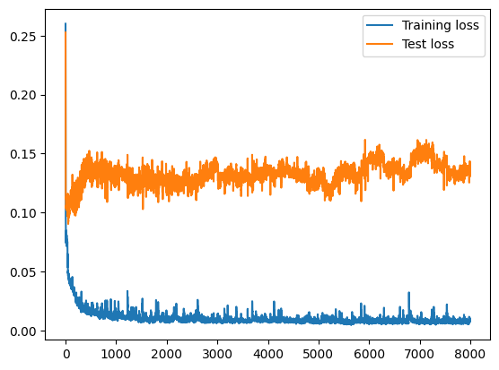
Train the data
# number of epochs to train the data
epochs = 8000

# empty list to store the performance of the model
train_history =[]
test_history =[]

# Training loop
for epoch in range(epochs):
    total_loss = 0.0

    # Training
    model.train()
    for batch_X, batch_y in train_loader:
        # reset the gradient for current loop
        optimizer.zero_grad()

        batch_X, batch_y = batch_X.to(device), batch_y.to(device)
        # predict the train data
        predictions = model(batch_X)
        # calculate the loss
        loss = loss_fn(predictions, batch_y)
        # calculate gradient
        loss.backward()
        # update the parameter based on the gradient and optimizer
        optimizer.step()

        total_loss += loss.item()

    # Calculate average training loss and accuracy
    average_loss = total_loss / len(train_loader)
    train_history.append(average_loss)

    # Validation on test data
    model.eval()
    with torch.no_grad():
        total_test_loss = 0.0

        for batch_X_test, batch_y_test in test_loader:
            batch_X_test, batch_y_test = batch_X_test.to(device), batch_y_test.to(device)
            # predict the test data
            predictions_test = model(batch_X_test)
            # calculate the loss
            test_loss = loss_fn(predictions_test, batch_y_test)

            total_test_loss += test_loss.item()

        # Calculate average test loss and accuracy
        average_test_loss = total_test_loss / len(test_loader)
        test_history.append(average_test_loss)

    if (epoch+1)%100==0:
        print(f'Epoch [{epoch+1}/{epochs}] - Training Loss: {average_loss:.4f}, Test Loss: {average_test_loss:.4f}')
Epoch [100/8000] - Training Loss: 0.0386, Test Loss: 0.1136
Epoch [200/8000] - Training Loss: 0.0280, Test Loss: 0.1130
Epoch [300/8000] - Training Loss: 0.0178, Test Loss: 0.1246
Epoch [400/8000] - Training Loss: 0.0170, Test Loss: 0.1291
Epoch [500/8000] - Training Loss: 0.0133, Test Loss: 0.1361
Epoch [600/8000] - Training Loss: 0.0152, Test Loss: 0.1401
Epoch [700/8000] - Training Loss: 0.0113, Test Loss: 0.1298
Epoch [800/8000] - Training Loss: 0.0141, Test Loss: 0.1302
Epoch [900/8000] - Training Loss: 0.0180, Test Loss: 0.1425
Epoch [1000/8000] - Training Loss: 0.0111, Test Loss: 0.1330
Epoch [1100/8000] - Training Loss: 0.0111, Test Loss: 0.1327
Epoch [1200/8000] - Training Loss: 0.0107, Test Loss: 0.1298
Epoch [1300/8000] - Training Loss: 0.0142, Test Loss: 0.1165
Epoch [1400/8000] - Training Loss: 0.0118, Test Loss: 0.1204
Epoch [1500/8000] - Training Loss: 0.0089, Test Loss: 0.1262
Epoch [1600/8000] - Training Loss: 0.0108, Test Loss: 0.1380
Epoch [1700/8000] - Training Loss: 0.0097, Test Loss: 0.1245
Epoch [1800/8000] - Training Loss: 0.0119, Test Loss: 0.1208
Epoch [1900/8000] - Training Loss: 0.0121, Test Loss: 0.1355
Epoch [2000/8000] - Training Loss: 0.0107, Test Loss: 0.1317
Epoch [2100/8000] - Training Loss: 0.0096, Test Loss: 0.1214
Epoch [2200/8000] - Training Loss: 0.0105, Test Loss: 0.1190
Epoch [2300/8000] - Training Loss: 0.0079, Test Loss: 0.1257
Epoch [2400/8000] - Training Loss: 0.0094, Test Loss: 0.1289
Epoch [2500/8000] - Training Loss: 0.0082, Test Loss: 0.1216
Epoch [2600/8000] - Training Loss: 0.0092, Test Loss: 0.1307
Epoch [2700/8000] - Training Loss: 0.0096, Test Loss: 0.1322
Epoch [2800/8000] - Training Loss: 0.0082, Test Loss: 0.1319
Epoch [2900/8000] - Training Loss: 0.0101, Test Loss: 0.1348
Epoch [3000/8000] - Training Loss: 0.0079, Test Loss: 0.1361
Epoch [3100/8000] - Training Loss: 0.0071, Test Loss: 0.1275
Epoch [3200/8000] - Training Loss: 0.0076, Test Loss: 0.1282
Epoch [3300/8000] - Training Loss: 0.0067, Test Loss: 0.1351
Epoch [3400/8000] - Training Loss: 0.0096, Test Loss: 0.1276
Epoch [3500/8000] - Training Loss: 0.0086, Test Loss: 0.1331
Epoch [3600/8000] - Training Loss: 0.0183, Test Loss: 0.1310
Epoch [3700/8000] - Training Loss: 0.0148, Test Loss: 0.1270
Epoch [3800/8000] - Training Loss: 0.0079, Test Loss: 0.1313
Epoch [3900/8000] - Training Loss: 0.0081, Test Loss: 0.1335
Epoch [4000/8000] - Training Loss: 0.0076, Test Loss: 0.1389
Epoch [4100/8000] - Training Loss: 0.0080, Test Loss: 0.1355
Epoch [4200/8000] - Training Loss: 0.0077, Test Loss: 0.1347
Epoch [4300/8000] - Training Loss: 0.0073, Test Loss: 0.1429
Epoch [4400/8000] - Training Loss: 0.0074, Test Loss: 0.1381
Epoch [4500/8000] - Training Loss: 0.0088, Test Loss: 0.1336
Epoch [4600/8000] - Training Loss: 0.0070, Test Loss: 0.1340
Epoch [4700/8000] - Training Loss: 0.0065, Test Loss: 0.1345
Epoch [4800/8000] - Training Loss: 0.0072, Test Loss: 0.1281
Epoch [4900/8000] - Training Loss: 0.0068, Test Loss: 0.1231
Epoch [5000/8000] - Training Loss: 0.0066, Test Loss: 0.1321
Epoch [5100/8000] - Training Loss: 0.0080, Test Loss: 0.1373
Epoch [5200/8000] - Training Loss: 0.0088, Test Loss: 0.1182
Epoch [5300/8000] - Training Loss: 0.0089, Test Loss: 0.1265
Epoch [5400/8000] - Training Loss: 0.0075, Test Loss: 0.1313
Epoch [5500/8000] - Training Loss: 0.0073, Test Loss: 0.1329
Epoch [5600/8000] - Training Loss: 0.0053, Test Loss: 0.1385
Epoch [5700/8000] - Training Loss: 0.0093, Test Loss: 0.1265
Epoch [5800/8000] - Training Loss: 0.0067, Test Loss: 0.1320
Epoch [5900/8000] - Training Loss: 0.0064, Test Loss: 0.1418
Epoch [6000/8000] - Training Loss: 0.0064, Test Loss: 0.1475
Epoch [6100/8000] - Training Loss: 0.0065, Test Loss: 0.1467
Epoch [6200/8000] - Training Loss: 0.0063, Test Loss: 0.1501
Epoch [6300/8000] - Training Loss: 0.0096, Test Loss: 0.1354
Epoch [6400/8000] - Training Loss: 0.0092, Test Loss: 0.1371
Epoch [6500/8000] - Training Loss: 0.0058, Test Loss: 0.1376
Epoch [6600/8000] - Training Loss: 0.0062, Test Loss: 0.1398
Epoch [6700/8000] - Training Loss: 0.0099, Test Loss: 0.1281
Epoch [6800/8000] - Training Loss: 0.0128, Test Loss: 0.1373
Epoch [6900/8000] - Training Loss: 0.0073, Test Loss: 0.1480
Epoch [7000/8000] - Training Loss: 0.0077, Test Loss: 0.1587
Epoch [7100/8000] - Training Loss: 0.0061, Test Loss: 0.1566
Epoch [7200/8000] - Training Loss: 0.0083, Test Loss: 0.1505
Epoch [7300/8000] - Training Loss: 0.0070, Test Loss: 0.1409
Epoch [7400/8000] - Training Loss: 0.0087, Test Loss: 0.1443
Epoch [7500/8000] - Training Loss: 0.0063, Test Loss: 0.1405
Epoch [7600/8000] - Training Loss: 0.0071, Test Loss: 0.1330
Epoch [7700/8000] - Training Loss: 0.0066, Test Loss: 0.1323
Epoch [7800/8000] - Training Loss: 0.0074, Test Loss: 0.1371
Epoch [7900/8000] - Training Loss: 0.0063, Test Loss: 0.1345
Epoch [8000/8000] - Training Loss: 0.0088, Test Loss: 0.1309
# visualize the train and test loss
plt.plot(train_history, label="Training loss")
plt.plot(test_history, label="Test loss")
plt.legend()
plt.show()
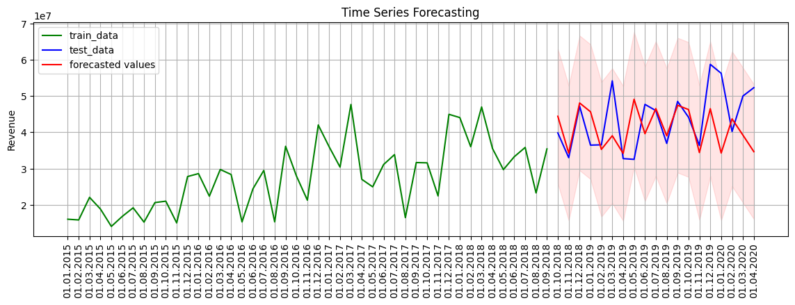
# Define the number of future time steps to forecast
num_forecast_steps = 19

# Convert to NumPy and remove singleton dimensions
sequence_to_plot = X_train.squeeze().cpu().numpy()

# Use the last data points as the starting point
historical_data = sequence_to_plot[-1]

# Initialize a list to store the forecasted values
forecasted_values = []

last_two_value = []

# Use the trained model to forecast future values
with torch.no_grad():
    for _ in range(num_forecast_steps):
        # Prepare the previous points as tensor
        historical_data_tensor = torch.as_tensor(historical_data).view(1, -1, 1).float().to(device)
        # Predict the next revenue
        predicted_value = model(historical_data_tensor).cpu().numpy()[0, 0]

        # Append the predicted value to the forecasted_values list
        forecasted_values.append(predicted_value[0])

        # Update the historical_data sequence by removing the oldest value and adding the predicted value
        historical_data = np.roll(historical_data, shift=-1)
        historical_data[-1] = predicted_value
#set the size of the plot
plt.rcParams['figure.figsize'] = [14, 4]

# Train data
plt.plot(train_index, data[:train_len], label = "train_data", color = "g")

# Test data
plt.plot(test_index, data[train_len:], label = "test_data", color = "b")

# Calculate the confidence interval of the prediction
rmse = np.sqrt(average_test_loss)
se = 1.96*rmse
upper_bound = [x+se for x in forecasted_values]
lower_bound = [x-se for x in forecasted_values]

#Forecasted Values
#reverse the scaling transformation
forecasted_cases = scaler.inverse_transform(np.expand_dims(forecasted_values, axis=0)).flatten()
upper_bound = scaler.inverse_transform(np.expand_dims(upper_bound, axis=0)).flatten()
lower_bound = scaler.inverse_transform(np.expand_dims(lower_bound, axis=0)).flatten()
# plotting the forecasted values
plt.plot(test_index, forecasted_cases, label='forecasted values', color='red')
plt.fill_between(test_index, lower_bound, upper_bound, color='red', alpha=0.1)

plt.ylabel('Revenue')
plt.legend()
plt.xticks(rotation=90)
plt.title('Time Series Forecasting')
plt.grid(True)